Moving From Stocks to Bonds: Time Segmentation and Glide Paths

Introduction

Common investment practice holds that investment time span should be a significant factor when determining portfolio asset allocation based on risk tolerance. The longer the investment time span, the more aggressive the asset allocation can be, while a short investment time span requires a more conservative strategy.

This article looks at the financial effects of moving between stocks and bonds over the course of an investment time span. The most common strategies of time segmentation and glide paths are compared with static asset allocations.

Methodology

Two possible investments are considered:

• Large cap U.S. stocks with an average annual return of 11.86% and a standard deviation of 19.40% based on the performance of 1928-2025.
• Risk-free bonds with an annual return of 5%.

The bond holdings are simplified to not have any interest rate risk or reinvestment risk. The yield curve is also assumed to be flat. This simplification causes the exact numbers to be different from a more realistic model, but it does not have a significant impact on the comparisons being made.

Ten thousand simulations are run with the results sorted into percentiles by portfolio ending balance. All portfolios being compared run simultaneously for each simulation so that they are compared based on the same sequences of stock returns. Each portfolio has a starting balance of 1.

The results are presented as graphs of ending portfolio balances at each percentile. The graphs are arbitrarily truncated at the 98th percentile to prevent the very highest percentiles from taking up the majority of the vertical space on the graphs.

No consideration is made with regard to accumulation or decumulation. Since the processes of accumulation and decumulation can be deconstructed into tranches of funds with specific dates when they are saved matched up with liabilities with specific dates when the tranches are meant to be spent, each individual tranche would have a single investment time span as explored in this article.

Stocks, Bonds, and Investment Time Span

To begin, it is worth comparing the effect that different time spans have on portfolios consisting of either 100% stocks or 100% bonds.

Figure 1 - Stocks vs Bonds - 10 years (Full Size)

Figure 2 - Stocks vs Bonds - 20 years (Full Size)

Figure 3 - Stocks vs Bonds - 40 years (Full Size)

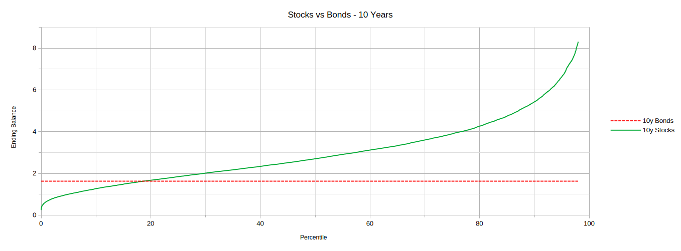
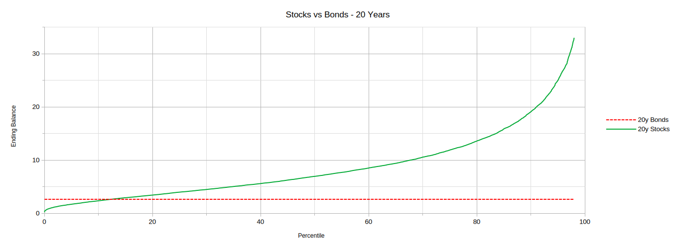
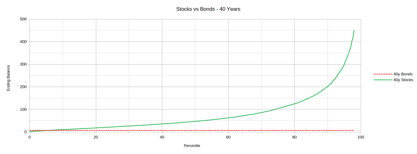
There are two notable features seen in these three figures. First, longer time spans increase both the probability and the relative magnitude of the upside versus the downside of stocks compared with bonds. Second, even though longer time spans reduce the probability of stocks underperforming bonds, the worst-case result still remains sharply lower for stocks no matter the length of time.

Time Segmentation

Next, we look at time segmentation, also known as the bucket strategy. The first version to be examined is dividing up a 10 year investment into 5 years of 100% stocks followed by 5 years of 100% bonds. Figures 4 & 5 show the results.

Figure 4 - Time Segmentation (0-10th Percentile) - 10 years (Full Size)

Figure 5 - Time Segmentation (Full Results) - 10 years (Full Size)

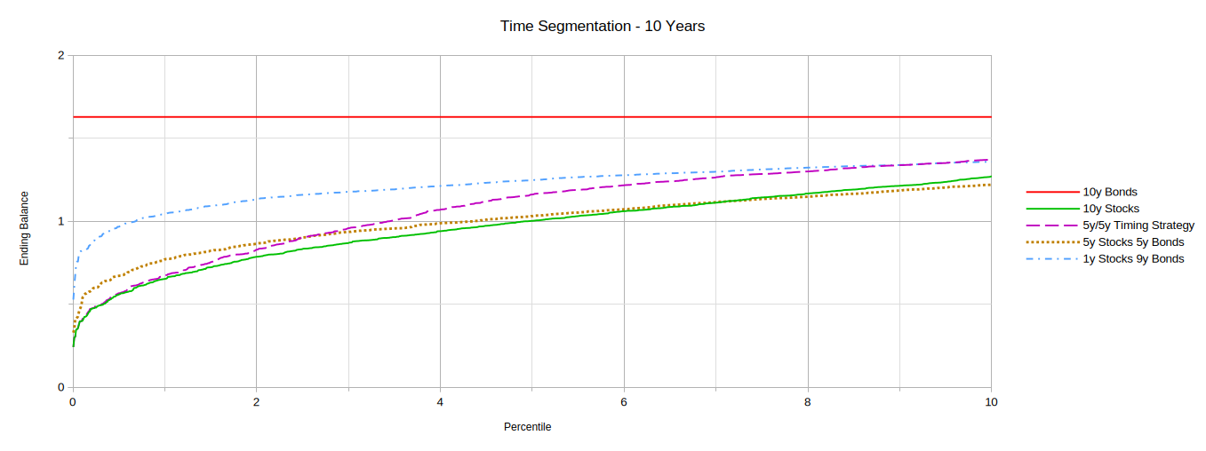
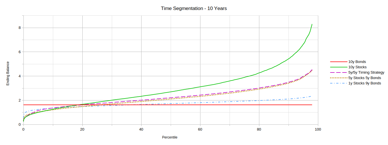
The results show a large drop in the upside compared with stocks while only offering a slight benefit in the lowest percentiles. The reason for this poor performance is best explained by looking at the "1 year stocks, 9 year bonds" strategy also shown in the figures. Of particular note is that having the funds invested in stocks even for a single year increases the downside risk by over half of the difference between entirely bonds and entirely stocks. Putting the funds into stocks for five years is only slightly less risky than keeping them there for the full ten years. This shows that each additional year the funds remain invested in stocks adds sharply less risk than the last, although there is always some additional risk.

Bucket strategies usually follow a rule that prevents "selling stocks when they are down." Figures 4 & 5 also consider such a timing rule. The "5 year, 5 year timing strategy" also invests for 5 years in 100% stocks but only switches over to 100% bonds if the stocks are at a new high compared to all prior years. If the stocks never make new highs, this can lead to the portfolio remaining in 100% stocks for the full 10 years which is evident in the timing strategy results matching the worst-case performance of the 10 year stock portfolio. The timing strategy does lead to somewhat better results compared with the mechanical "5 year stocks, 5 year bonds" strategy except at the lowest percentiles.

The following figures compare the results of static asset allocations with the time segmentation strategy. Two allocations are considered:

• A diversified 60% stocks, 40% bonds portfolio with annual rebalancing, and
• A similar 60% stocks and 40% bonds portfolio, except the stocks and bonds are "split" so that they don't interact with each other (no rebalancing).

Figure 6 - Static Asset Allocation (0-10th Percentile) - 10 years (Full Size)

Figure 7 - Static Asset Allocation (Full Results) - 10 years (Full Size)

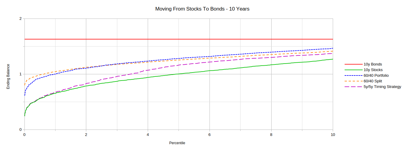
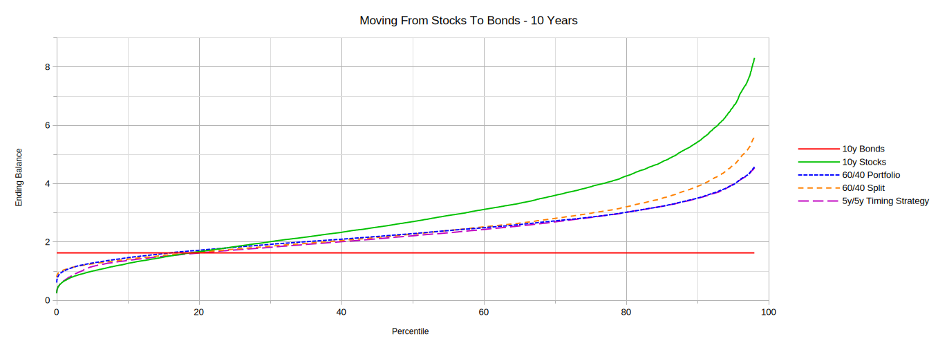
Figures 6 & 7 show that the split portfolio is always at least as good as the time segmentation strategy, significantly outperforming it at both the lowest and highest percentiles. The rebalanced portfolio also is always at least a match for the time segmentation strategy, starting with a significant edge at the lowest percentiles and continuing with a slight advantage until the higher percentiles.

Comparing the split and rebalanced portfolios, rebalancing is slightly superior in the percentiles where the average stock returns are fairly close to the bond returns. This is the benefit of diversification. The rebalanced portfolio underperforms in the worst-case percentiles due to funds transferred from the bond portion being dragged down by continuously poor stock performance. The split portfolio also outperforms the rebalanced portfolio in the higher percentiles when the stocks are allowed to grow freely without being tethered to a bond anchor.

Extending the investment time span to 20 years is also considered. In this case, the time segmentation strategy is extended to "15 years stocks, 5 years bonds" while the static asset allocations are changed to 80% stocks and 20% bonds.

Figure 8 - Static Asset Allocation (0-10th Percentile) - 20 years (Full Size)

Figure 9 - Static Asset Allocation (Full Results) - 20 years (Full Size)

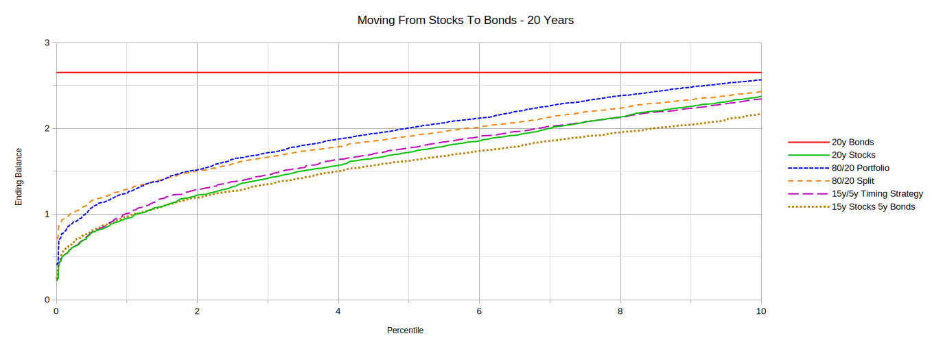
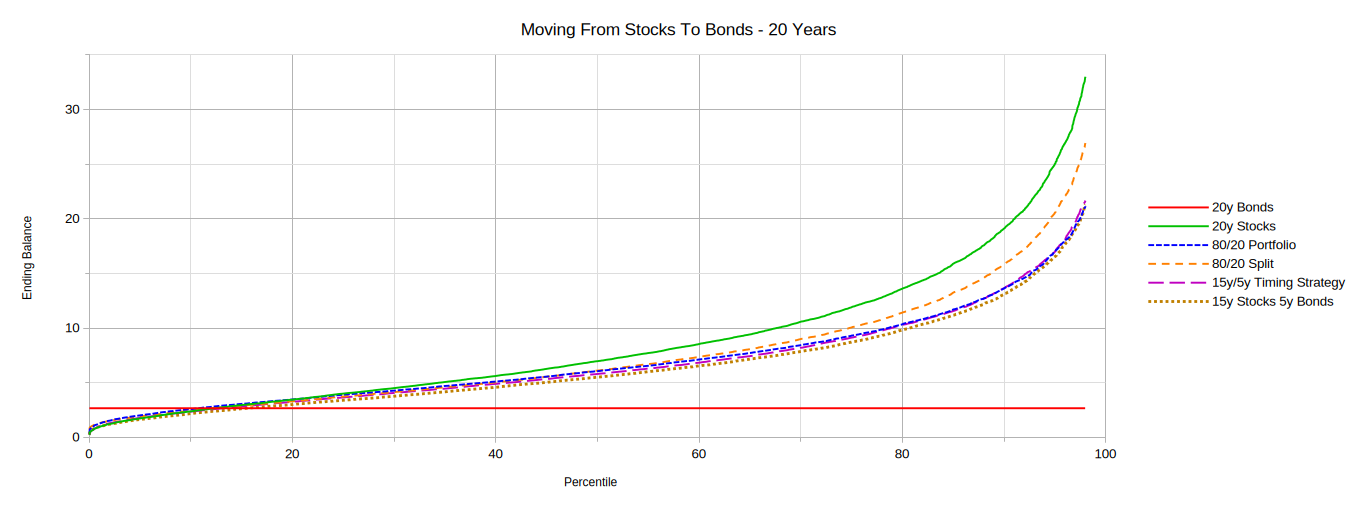
Figures 8 & 9 show that any benefit of the two time segmentation strategies compared to a 100% stock strategy virtually disappears at this longer time span while the loss of upside remains substantial. The static asset allocation strategies perform similarly to the 10 year time span results other than differences due to the increased stock allocations.

Glide Paths

A glide path is the practice of transitioning a diversified portfolio from one asset allocation to a different asset allocation over a period of time. This is commonly used in retirement planning and is a key feature of target date mutual funds and ETFs. Typically, a glide path starts with an aggressive asset allocation of mostly stocks and ends with a conservative asset allocation of mostly bonds.

First, we consider a 10 year investment time span. The glide path starts with an asset allocation of 90% stocks and 10% bonds in the first year and ends with an asset allocation of 30% stocks and 70% bonds in the tenth year. The asset allocation is annually rebalanced in a linear fashion between those two allocations in the intervening years. A static diversified portfolio with an asset allocation of 64% stocks and 36% bonds that is annually rebalanced is used for comparison.

Figure 10 - Glide Path (0-10th Percentile) - 10 years (Full Size)

Figure 11 - Glide Path (Full Results) - 10 years (Full Size)

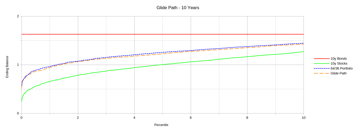
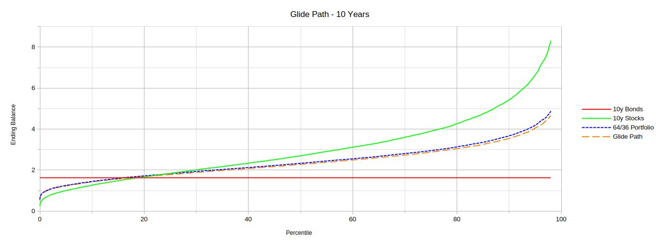
Figures 10 & 11 show that there is very little difference in the results between the glide path portfolio and the static portfolio. The static portfolio has the same or slightly better results at ever percentile.

Next, we consider a 20 year investment time span. The glide path starts with an asset allocation of 90% stocks and 10% bonds in the first year and ends with an asset allocation of 30% stocks and 70% bonds in the twentieth year. The asset allocation is annually rebalanced in a linear fashion between those two allocations in the intervening years. A static diversified portfolio with an asset allocation of 62% stocks and 38% bonds that is annually rebalanced is used for comparison.

Figure 12 - Glide Path (0-10th Percentile) - 20 years (Full Size)

Figure 13 - Glide Path (Full Results) - 20 years (Full Size)

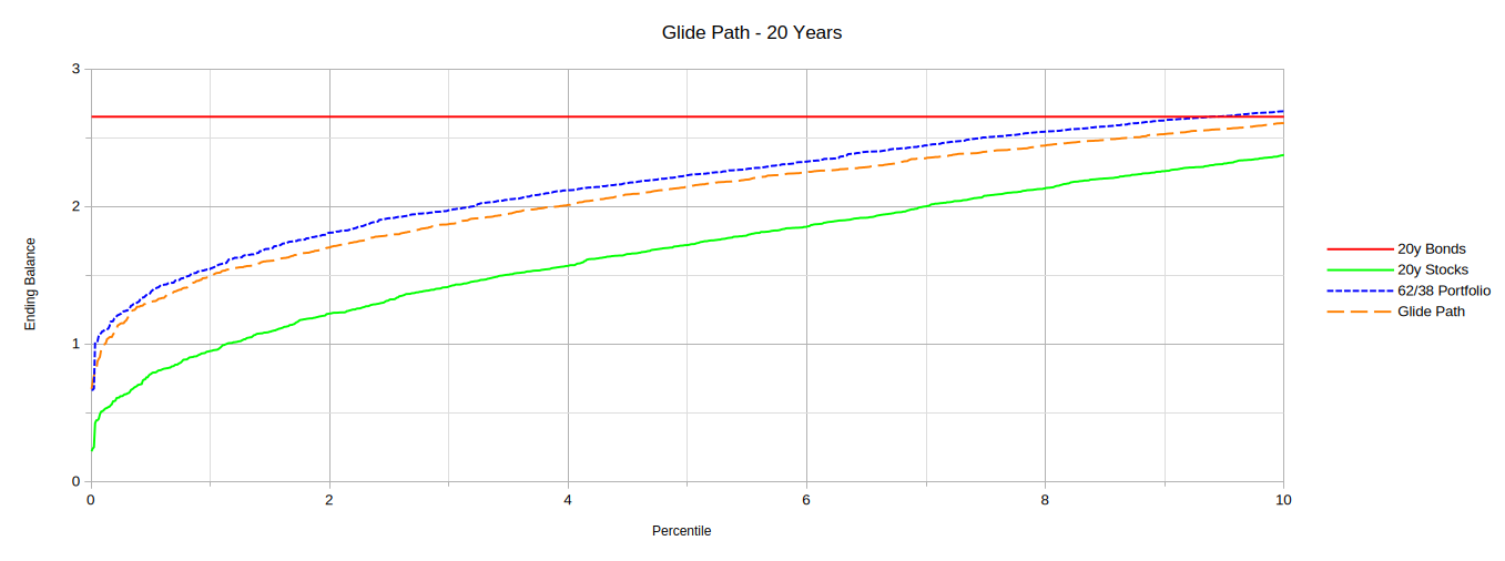
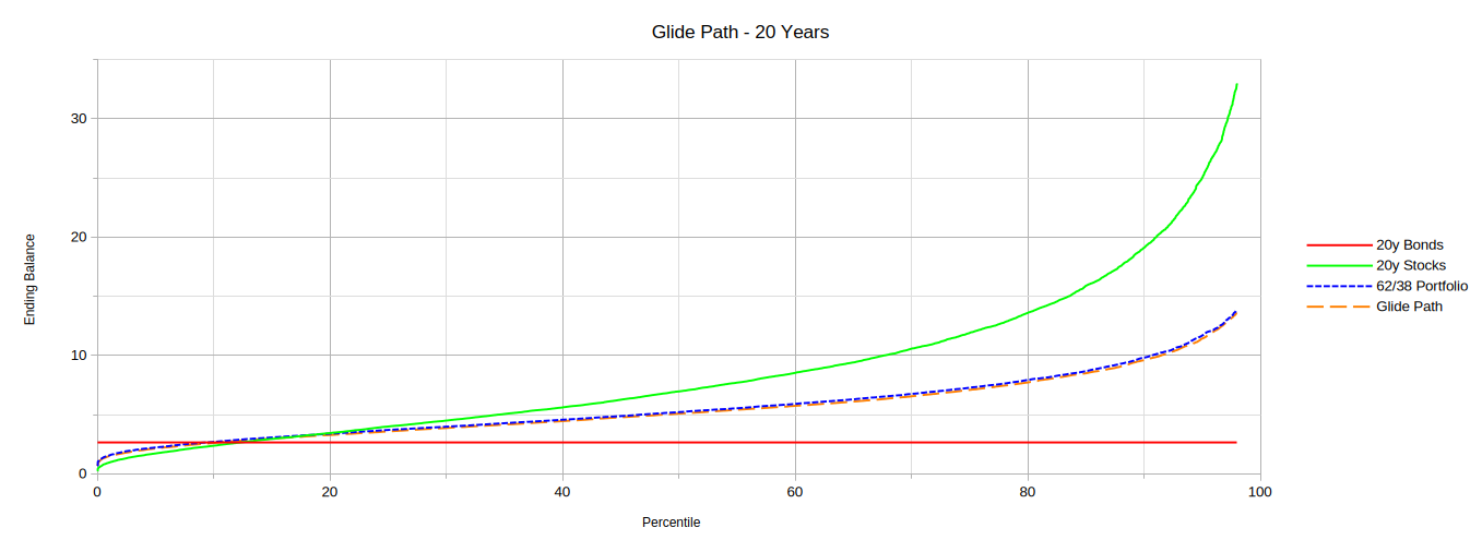
Figures 12 & 13 show that again there is very little difference in the results between the glide path portfolio and the static portfolio. The static portfolio still has the same or slightly better results at ever percentile.

Finally, we consider a 40 year investment time span. The glide path starts with an asset allocation of 90% stocks and 10% bonds for the first 20 years that is annually rebalanced. The glide path starts adjusting in the 21st year and ends with an asset allocation of 30% stocks and 70% bonds in the fortieth year. The asset allocation is annually rebalanced in a linear fashion between those two allocations in the intervening years. A static diversified portfolio with an asset allocation of 60% stocks and 40% bonds that is annually rebalanced is used for comparison.

Figure 14 - Glide Path (0-10th Percentile) - 40 years (Full Size)

Figure 15 - Glide Path (Full Results) - 40 years (Full Size)

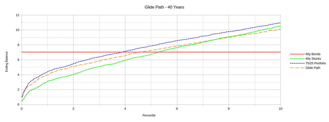
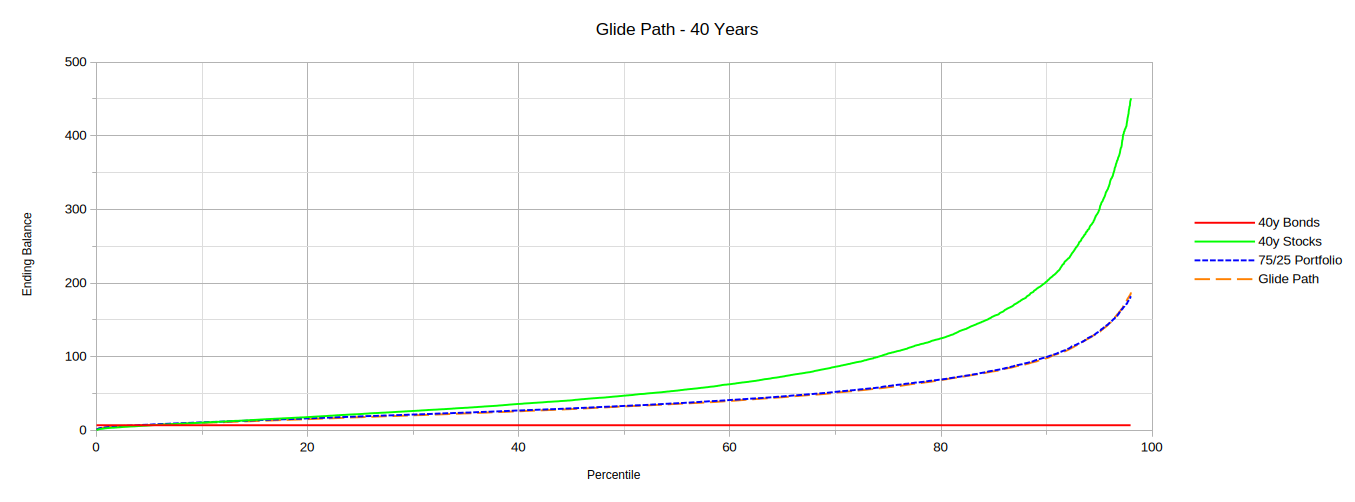
Figures 14 & 15 show that once again there is very little difference in the results between the glide path portfolio and the static portfolio with the static portfolio often having a slight edge.

Analysis

Based on the preceding results, adjusting portfolio asset allocations within an investment time span leads to inferior financial results compared to alternatives. The two strategies that offer the optimal solutions for managing the trade-offs between the risk management of bonds and the rewards of stocks are a diversified rebalanced portfolio and a split portfolio approach.

The diversified portfolio that is periodically rebalanced offers the traditional approach. It provides the best results of the strategies considered when faced with below average market returns. This offers the smoothest result for an investor with moderate risk tolerance. However, it supplies no guarantee for achieving a minimum ending balance in the worst-case percentiles, only a minimum probability of achieving such an ending balance.

The split portfolio approach allows the liabilities to be further deconstructed into either essential (fixed) liabilities or discretionary (flexible) liabilities. (In fact, what might be a single liability can be divided into essential and discretionary portions.) An essential liability can be met with a 100% bond portfolio and a discretionary liability can be met with a 100% stock portfolio. Such a division allows essential liabilities to receive a guaranteed funding amount while discretionary liabilities receive the maximum funding that the market will provide. This matches the strengths of the split portfolio approach: the best results for both the worst-case percentiles and above average market returns.

The preceding results also show that stock portfolios benefit much more from longer investment time spans than bond portfolios do. This suggests that 100% stock portfolios funding discretionary liabilities should be saved for first while 100% bond portfolios funding essential liabilities should be saved for last. This might appear similar to time segmentation or a glide path, but it is fundamentally different in that the stocks are kept separate from the bonds and remain fully invested for the entire investment time span.

Conclusion

The results of this research show that investment strategies that involve transitioning from stocks to bonds over time offer no financial benefits. In fact they often significantly underperform static asset allocations. The five main findings of this research are as follows:

First, both the fixed year time segmentation strategy and the "sell at new highs" time segmentation strategy produce inferior results compared to static asset allocations.

Second, glide paths produce results that are slightly worse than a corresponding static asset allocation.

Third, investing in stocks for even a single year introduces a significant amount of risk to the overall returns. The only method for avoiding that risk is to never invest in stocks.

Fourth, investing in a diversified rebalanced portfolio has greater worst-case risk than keeping the stocks and bonds separate.

Finally, the longer the investment time span, the more compelling the argument is to invest in 100% stocks for maximum (yet uncertain) returns. On the other hand, the argument for bonds goes completely in reverse: the more certain the investment result needs to be, the more appropriate it is to invest in 100% bonds over as short an investment time span as possible.